Equation Driven Curve

Enter the equation into the sketch to create the corresponding curve.

---

How to use it:

1.Click equation curve command, pop-up dialog box.

2.Type of equation: There are two kinds of "dominant, parametric". Default dominance.

3.Type of coordinate system: There are two kinds of "Cartesian, polar coordinates". Default Cartesian.

4.Equation: Enter the equation to generate the corresponding curve. You can use the "Equation Library" feature to quickly insert saved equations.

Types of equations	Coordinate system type	Input box	Prompt when the mouse points to the input box
Dominance	Descartes	y=	Enter an equation that takes x as an argument, such as 3*sin(x)+1
	Polar Coordinates	β=	Enter an equation that takes t as an argument, such as 3*sin(t)+1
Parametric	Descartes	y=	Enter an equation that takes t as an argument, such as 3*sin(t)+1
		x=	Enter an equation that takes t as an argument, such as 3*sin(t)+1
	Polar Coordinates	β=	Enter an equation that takes t as an argument, such as 3*sin(t)+1
		θ=	Enter an equation that takes t as an argument, such as 3*sin(t)+1

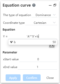
Enter variable equations, you can enter equations with variables created through the "Variable Management" function, which automatically updates variable parameters in the equation curve when the features associated with the variable change.

• Enter the variable name in the input field and the available variables will be displayed in the drop down box.

• Mouse click on the variable in the drop-down box to reference this variable in that input box.

• When the value of this variable is modified, the equation curve will be updated automatically.

5. Parameters: Enter the starting/ending values of x or t to generate a curve in the range of the starting and ending values. Default to null.

• Start and end values are not equal.
• The default insertion point of the curve is the coordinate point corresponding to the starting value.

6.An equation curve has the same effect of adding constraints as a spline curve.

7.Click on the already generated curve to bring up the Properties dialog box. You can edit the equation or other parameters.

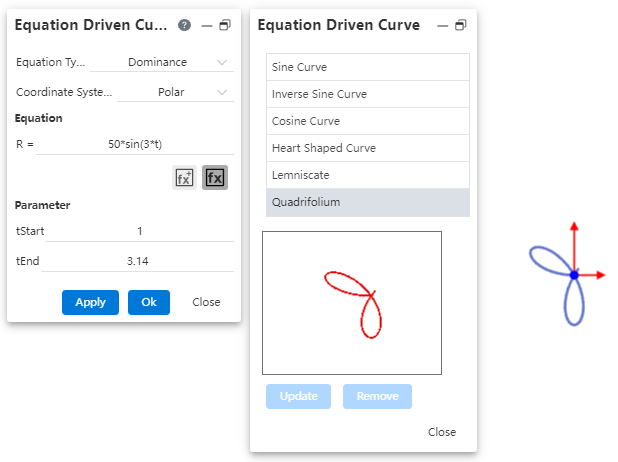
Equation Library

You can insert an existing equation in the sketch library, or add a custom equation to the equation library for quick subsequent calls;

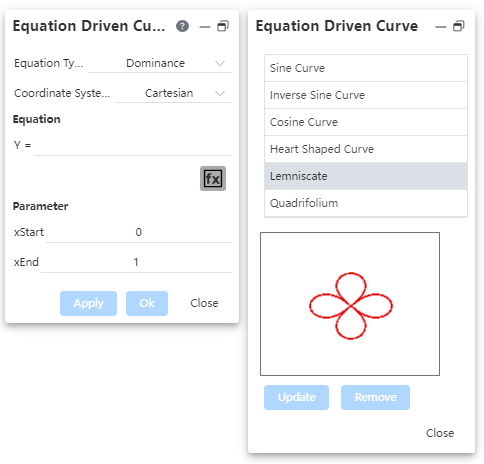
• Example of calling equations:

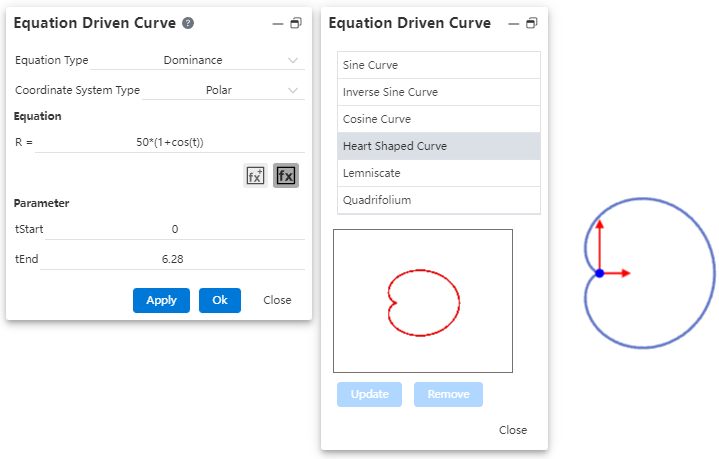
Double click an equation in the equation list to fill it into the left Equation dialog box and support direct participation in modeling. Can be previewed in the viewport:

Equation parameters can be adjusted to generate a new equation curve:

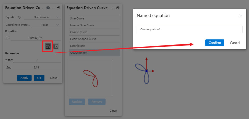
1）To save a custom equation:

After filling in the equation, click to add the equation to the equation library, and return to the corresponding list according to the equation type;